Full-Stack Load Testing on Windows 11: Building a k6 + Docker + Prometheus + Grafana Observability Pipeline

In a previous post, I built a lightweight load testing pipeline using k6, Flask, psutil and Plotly — no Docker, no databases, no running services. It worked well for quick ad-hoc testing, but it had a fundamental limitation: you couldn’t see what was happening during the test. You had to wait for the test to finish, then generate a static HTML dashboard. For a 3-minute load test that’s fine. For a 20-minute stress test where you want to watch the server buckle in real-time, it’s not.

This post describes the next evolution: a full observability stack using Docker Compose, Prometheus, InfluxDB, Grafana and windows_exporter that streams metrics in real-time to a professional dashboard — all running across two Windows 11 machines on a home network.

The full project is available on GitHub.

What This Solution Does

The stack splits across two machines:

Remote machine (the server being tested) runs everything inside Docker:

A Flask application — the Application Under Test (AUT) with Prometheus instrumentation
Prometheus — scraping metrics from both the Flask app and the host OS every 5 seconds
InfluxDB — receiving k6 performance data in real-time via the InfluxDB line protocol
Grafana — rendering a pre-built dashboard that combines all three data sources

Outside Docker, windows_exporter runs as a native Windows service, exposing CPU, memory, disk and network metrics on port 9182.

Local machine (the load generator) runs only k6. No Docker, no Python, no services — just:

k6 run --out influxdb=http://REMOTE_IP:8086/k6 -e BASE_URL=http://REMOTE_IP:5000 load_test.js

The --out influxdb flag is the key. k6 writes every metric — response times, request counts, virtual user counts, data transferred — directly into InfluxDB on the remote machine in real-time. Open the Grafana dashboard in a browser and you see the data flowing as the test runs.

The Architecture

LOCAL MACHINE              REMOTE MACHINE (Docker)
+-----------+              +----------------------------+
|           | HTTP reqs    | Flask AUT (:5000)          |
| k6        | -----------> | /metrics (Prometheus)      |
|           |              |                            |
| --out     | InfluxDB     | InfluxDB (:8086)           |
| influxdb  | -----------> | database: k6               |
|           |              |                            |
+-----------+              | Prometheus (:9090)         |
                           | <- scrapes Flask /metrics  |
  Browser                  | <- scrapes windows_exporter|
+-----------+              |                            |
| Grafana   | <----------> | Grafana (:3000)            |
| Dashboard | port 3000    | <- queries InfluxDB        |
+-----------+              | <- queries Prometheus      |
                           +----------------------------+

                           NATIVE WINDOWS SERVICE
                           +----------------------------+
                           | windows_exporter (:9182)   |
                           | CPU, memory, disk, network |
                           +----------------------------+

The beauty of this design is the separation of concerns. Prometheus handles system and application metrics (CPU usage, memory, Flask request rates). InfluxDB handles k6 load test metrics (response times, virtual users, throughput). Grafana combines both on a shared time axis, so you can immediately see correlations — “response times spiked at 14:32, and CPU hit 95% at exactly the same moment.”

The Dashboard: Three Sections, Two Data Sources

The pre-built Grafana dashboard has three sections:

k6 Performance Metrics (from InfluxDB)

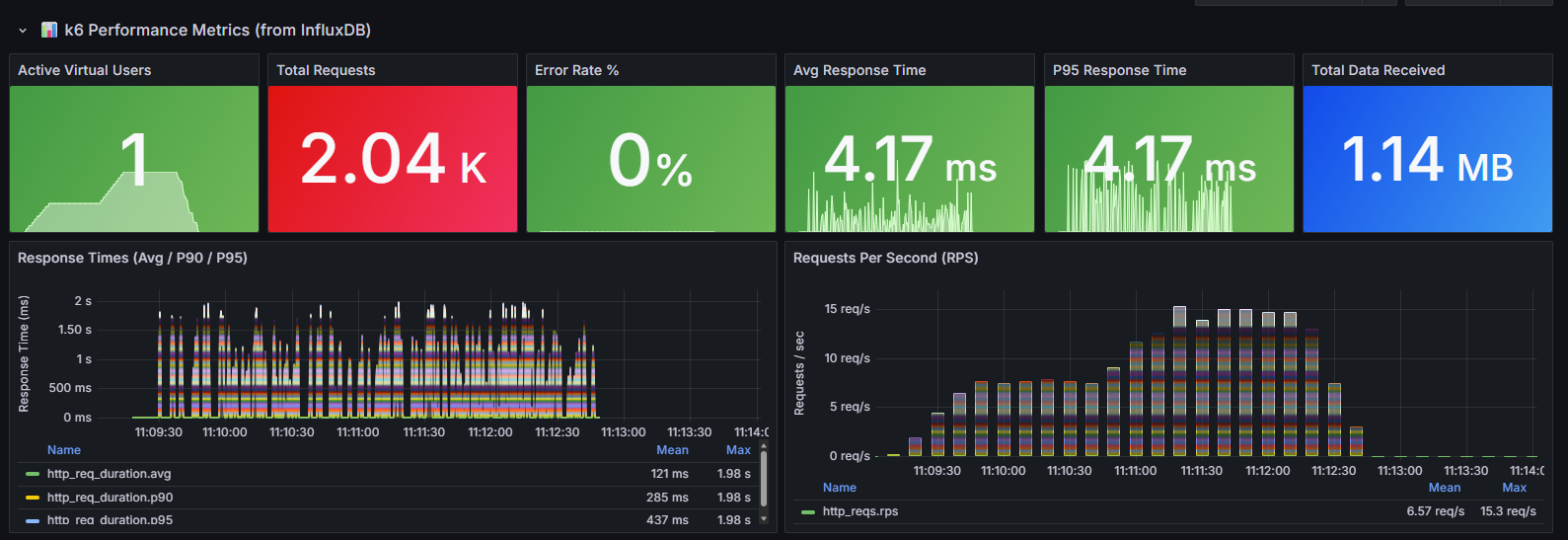
The top row contains six stat panels that give an at-a-glance summary of the test:

Active Virtual Users — the number of simulated users currently executing requests. The sparkline shows the ramp-up and ramp-down profile over the test duration. In this run, the test ramped up to 1 VU as a baseline check.
Total Requests — the cumulative count of HTTP requests made during the test (2.04K here). This tells you the overall volume of traffic generated.
Error Rate % — the percentage of requests that returned a non-2xx status code or timed out. 0% means every request succeeded — any value above 0% warrants investigation.
Avg Response Time — the arithmetic mean of all response durations (4.17ms). Useful as a general indicator, but can be misleading if the distribution is skewed by outliers.
P95 Response Time — the 95th percentile response time (4.17ms). This means 95% of all requests completed within this duration. P95 is a more reliable indicator of user experience than the average, because it captures the “worst case for most users” rather than being dragged down by the fast majority.
Total Data Received — the total bytes received from the server across all responses (1.14 MB). Useful for estimating bandwidth requirements under load.

Below the stat panels are two time-series charts:

Response Times (Avg / P90 / P95) — plots the average, 90th percentile and 95th percentile response times over the duration of the test. The spread between these lines reveals response time consistency — a tight grouping means predictable performance, while a wide spread indicates high variance. Here the P95 (blue) peaks around 1.5–2 seconds during the sustained phase, while the average (green) stays much lower around 100–500ms, indicating occasional slow responses.
Requests Per Second (RPS) — the throughput of the system over time, measured as completed HTTP requests per second. This chart shows how throughput scales as VUs increase. The stacked colours represent different request URLs. A plateau or drop in RPS while VUs are still increasing signals the server is reaching its capacity ceiling.

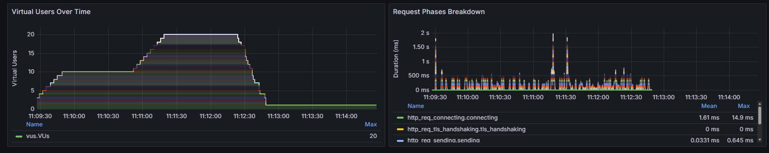
The second row continues with:

Virtual Users Over Time — shows the exact VU ramp profile across the test. This test used a staged ramp: climbing from 0 to 20 VUs in steps, holding at peak, then ramping back down. The stacked coloured lines represent individual VU threads. Correlating this chart with the response time chart above reveals exactly when performance starts degrading as load increases.
Request Phases Breakdown — decomposes each request’s total duration into its constituent phases: connecting (TCP handshake), TLS handshaking (SSL negotiation), sending (request upload), waiting (server processing time / time to first byte), and receiving (response download). This is critical for diagnosing where latency lives. Here, connecting averages 1.61ms with spikes to 14.9ms, TLS is 0ms (HTTP, not HTTPS), and sending is negligible at 0.03ms — meaning virtually all request time is spent waiting for the server to respond.

Windows System Metrics (from Prometheus via windows_exporter)

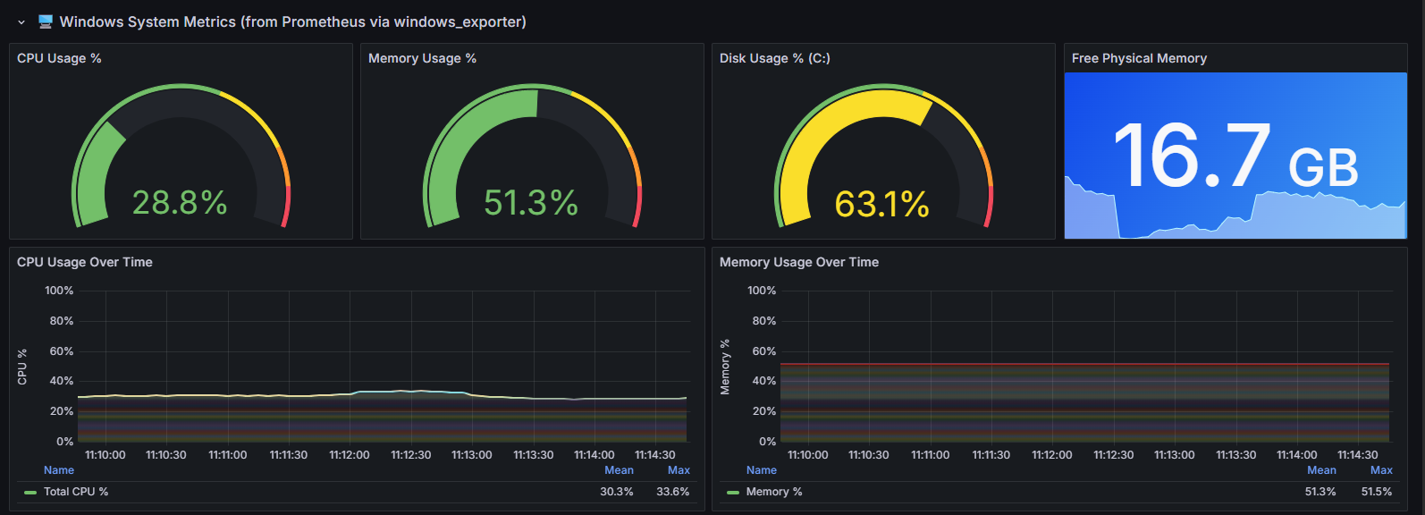
The top row shows four gauges providing instant readings of server resource utilisation:

CPU Usage % — current processor utilisation across all cores (28.8%). The colour coding shifts from green through yellow to red as utilisation increases. During load tests, watching this gauge tells you whether the server is CPU-bound. If it hits 90%+ while response times degrade, CPU is likely the bottleneck.
Memory Usage % — percentage of physical RAM currently in use (51.3%). High memory utilisation under load can indicate memory leaks, excessive caching, or simply undersized infrastructure. Sustained values above 85% risk triggering OS-level paging, which dramatically impacts response times.
Disk Usage % (C:) — the percentage of disk space consumed on the system volume (63.1%). While disk space rarely causes performance issues during a load test, running critically low can prevent logging, cause Docker containers to fail, or trigger system instability.
Free Physical Memory — the absolute amount of free RAM in gigabytes (16.7 GB). This complements the percentage gauge by showing the actual headroom available. A server showing 50% memory usage with 16.7 GB free has plenty of room; the same percentage on a 4 GB machine would be concerning.

Below the gauges:

CPU Usage Over Time — tracks processor utilisation across the full test duration. The green line (Total CPU %) averaged 30.3% with a peak of 33.6%, indicating the server was comfortably handling the load. A steadily climbing CPU line that doesn’t return to baseline after the test would suggest resource exhaustion or runaway processes.
Memory Usage Over Time — shows memory consumption stability. The flat line at ~51.3% (mean 51.3%, max 51.5%) confirms no memory leaks — the application allocated what it needed at startup and maintained a constant footprint throughout the test. A rising trend here would be a red flag.

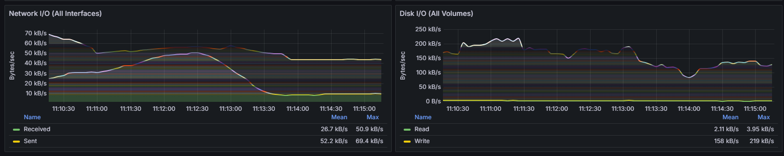
Network I/O (All Interfaces) — plots bytes sent and received per second across all network interfaces. The “Sent” line (yellow, mean 52.2 kB/s, max 69.4 kB/s) represents response data flowing back to the load generator, while “Received” (green, mean 26.7 kB/s, max 50.9 kB/s) represents incoming requests. The ratio between sent and received reveals the response-to-request size ratio. The visible correlation between network traffic and the VU ramp profile confirms that throughput scales proportionally with load.
Disk I/O (All Volumes) — tracks read and write throughput to disk. Write activity (yellow, mean 158 kB/s, max 219 kB/s) is significantly higher than reads (green, mean 2.11 kB/s, max 3.95 kB/s), which is expected — the writes come from Docker container logging, InfluxDB persisting metrics, and Prometheus writing its time-series database. The minimal read activity confirms the application is serving responses from memory rather than disk, which is ideal for low-latency performance.

Flask Application Metrics (from Prometheus)

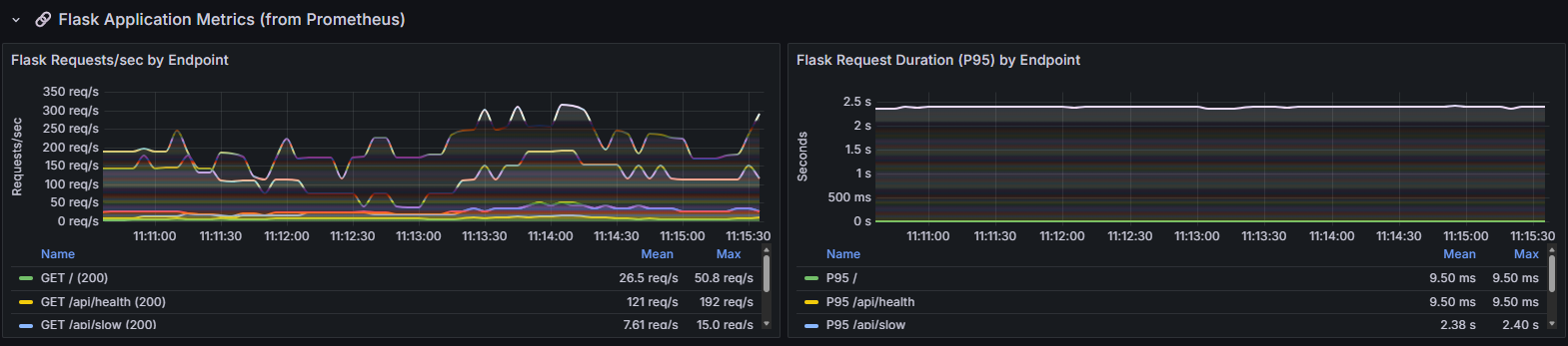
These panels show application-level metrics from the prometheus_client instrumentation embedded in the Flask app:

Flask Requests/sec by Endpoint — breaks down throughput per endpoint. The /api/health endpoint (yellow) handles the highest volume at a mean of 121 req/s (max 192 req/s), as k6 uses it for frequent health checks. The root endpoint / (green) averages 26.5 req/s (max 50.8 req/s), and /api/slow (blue) averages 7.61 req/s (max 15.0 req/s). The lower throughput on /api/slow is by design — it simulates a slow database query with a built-in delay. Watching how per-endpoint throughput changes under increasing load reveals which endpoints become bottlenecks first.
Flask Request Duration (P95) by Endpoint — shows the 95th percentile response time for each endpoint separately. The / and /api/health endpoints both maintain a stable P95 of 9.50ms throughout the test, confirming they’re fast and unaffected by load. The /api/slow endpoint shows a consistent P95 of ~2.38s (max 2.40s), matching its configured artificial delay. If this P95 were climbing over time rather than remaining flat, it would indicate the endpoint is degrading under sustained load — a sign of resource contention, connection pool exhaustion, or queue buildup.

The Flask App: Prometheus Instrumentation

Unlike the lightweight version where I used psutil to expose metrics via a custom /metrics endpoint, this version uses the standard prometheus_client Python library:

from prometheus_client import Counter, Histogram, Gauge, generate_latest

REQUEST_COUNT = Counter("flask_http_requests_total", "Total HTTP requests",
                        ["method", "endpoint", "status"])
REQUEST_DURATION = Histogram("flask_http_request_duration_seconds",
                             "HTTP request latency in seconds",
                             ["endpoint", "method"])
IN_PROGRESS = Gauge("flask_http_requests_in_progress",
                     "Number of HTTP requests currently being processed",
                     ["endpoint", "method"])

Middleware wraps every request automatically — tracking count, latency histogram and in-progress gauge per endpoint. The /metrics endpoint returns standard Prometheus exposition format, which Prometheus scrapes every 5 seconds.

The advantage over the psutil approach is that Prometheus owns the scraping. The Flask app doesn’t need to know anything about the monitoring infrastructure — it just exposes metrics in a standard format. If you swap Prometheus for Datadog or New Relic tomorrow, the app code doesn’t change.

Challenges: What Actually Went Wrong

Building this was not a smooth ride. Here are the real problems I hit, in the order I hit them.

Challenge 1: Grafana Datasource UID Binding

This was the most frustrating issue. The Grafana dashboard JSON references each datasource by a uid field:

{
  "datasource": { "type": "influxdb", "uid": "" }
}

When I first built the provisioning, I didn’t set explicit UIDs in datasources.yml. Grafana auto-generates UIDs for provisioned datasources, but the dashboard JSON had empty strings. Every single panel showed “No data” — even though data was flowing into both InfluxDB and Prometheus.

The fix was adding explicit uid fields to the datasource provisioning:

datasources:
  - name: Prometheus
    type: prometheus
    uid: prometheus-ds # ← explicit, matches dashboard JSON
    url: http://prometheus:9090

  - name: InfluxDB
    type: influxdb
    uid: influxdb-ds # ← explicit, matches dashboard JSON
    url: http://influxdb:8086
    database: k6

And referencing them in every panel:

{
  "datasource": { "type": "influxdb", "uid": "influxdb-ds" }
}

This is documented nowhere in the “getting started” guides. The Grafana provisioning docs mention UIDs in passing, but don’t explain that if your dashboard JSON references a UID that doesn’t match a provisioned datasource, the panel silently shows “No data” — no error message, no warning in the logs. You can spend hours checking whether Prometheus is scraping correctly or InfluxDB has data, when the problem is a string mismatch in a JSON file.

After fixing the files, you don’t even need to restart Grafana — the provisioning can be reloaded via API:

curl -X POST "http://REMOTE_IP:3000/api/admin/provisioning/datasources/reload" -u "admin:PASSWORD"
curl -X POST "http://REMOTE_IP:3000/api/admin/provisioning/dashboards/reload" -u "admin:PASSWORD"

Challenge 2: The Error Rate Panel

Even after fixing the datasource UIDs, the Error Rate % panel still showed “No data”. The original InfluxQL query was:

SELECT (sum("value") / (SELECT sum("value") FROM "http_reqs" WHERE $timeFilter)) * 100
FROM "http_req_failed"
WHERE $timeFilter AND "expected_response" = 'false'

The problem: when all requests succeed (0% error rate), k6 still writes records to http_req_failed — but the expected_response tag is "true" (meaning the response was expected/correct) and the value field is 0. The WHERE "expected_response" = 'false' clause filters out every record, returning nothing.

The fix was simplifying the query to use the value field directly:

SELECT mean("value") * 100 FROM "http_req_failed"
WHERE $timeFilter GROUP BY time($__interval) fill(null)

Since value is 0 for success and 1 for failure, mean * 100 gives the error percentage. This works correctly whether the error rate is 0%, 5%, or 100%.

Challenge 3: windows_exporter Inside vs Outside Docker

Prometheus runs inside Docker but needs to scrape windows_exporter running natively on the Windows host. Docker Desktop on Windows provides host.docker.internal as a DNS name that resolves to the host, but this required:

Setting extra_hosts: ["host.docker.internal:host-gateway"] in docker-compose.yml
Configuring the Prometheus scrape target as host.docker.internal:9182
Ensuring windows_exporter is installed as a Windows service with the right collectors enabled

The collector selection matters. Running windows_exporter with all default collectors generates thousands of metrics and the /metrics endpoint takes seconds to respond. Limiting to the collectors you actually need (cpu,cs,logical_disk,memory,net,os,process,system) keeps it fast and focused.

Challenge 4: UNC Paths and cmd.exe

The project lives on a network share (\\DESKTOP-M4R2VLU\Projects\K6FullStack), which means the workspace path is a UNC path. Windows cmd.exe cannot use UNC paths as working directories — it prints "UNC paths are not supported. Defaulting to Windows directory." and drops you into C:\Windows.

This means running k6 run scripts/load_test.js fails because k6 tries to resolve the path relative to C:\Windows. The workaround is using pushd which automatically maps a temporary drive letter to the UNC path:

pushd \\REMOTE\Projects\K6FullStack\local\scripts && k6 run load_test.js

pushd creates a temporary drive mapping (like Z:) and cds into it. When you popd, the drive mapping is removed. It’s one of those cmd.exe tricks that’s been around since Windows NT but nobody remembers.

The docker-compose.yml sets GF_SECURITY_ADMIN_PASSWORD=admin, but Grafana prompts you to change the password on first login. If you do change it (as you should), the default admin/admin credentials in all the documentation stop working — including for API calls like provisioning reloads. This caught me when I needed to reload the dashboard configuration remotely and curl -u admin:admin returned 401.

The lesson: either document the password change prominently, or use Grafana’s environment variable GF_SECURITY_DISABLE_INITIAL_ADMIN_CREATION to prevent the prompt (not recommended for anything beyond local testing).

Why InfluxDB 1.x, Not 2.x?

k6’s built-in --out influxdb output uses the InfluxDB 1.x line protocol natively. InfluxDB 2.x uses a completely different API (Flux query language, token-based auth, organisations and buckets instead of databases). Using InfluxDB 2.x with k6 requires either:

The xk6-output-influxdb extension (requires building k6 from source with xk6)
Or running an InfluxDB 2.x instance with the 1.x compatibility API enabled

Neither option is zero-configuration. InfluxDB 1.11 just works — start the container with INFLUXDB_DB=k6 and k6 writes to it immediately. For a load testing tool where you want results flowing in seconds, not hours of configuration, the 1.x simplicity wins.

Alternative Technologies: What Else Could Have Been Used

Load Testing Tools

Apache JMeter — The established enterprise choice. GUI-based test design with a massive plugin ecosystem. But JMeter uses XML test plans that are painful to version control, requires the JVM (significant resource overhead), and its per-VU memory consumption is roughly 10x that of k6. For scripting complex scenarios, k6’s JavaScript is far more readable than JMeter’s XML/BeanShell.

Locust — Python-based, which would have been a natural fit since the rest of the stack uses Python. Locust has a built-in web UI for real-time monitoring, distributed mode, and Python test scripts. The disadvantages: its built-in UI is real-time only (no historical data without an external store), per-VU overhead is higher than k6, and you’d still need the same Prometheus/InfluxDB/Grafana stack for persistent dashboards.

Gatling — Scala/Java-based with excellent HTML report generation. Strong choice for CI/CD pipelines. But the JVM dependency, Scala DSL learning curve, and resource overhead make it less appealing for a quick two-machine setup.

Metrics Storage

Prometheus Remote Write — Instead of InfluxDB, k6 could push directly to Prometheus using the xk6-output-prometheus-remote extension. This would eliminate InfluxDB entirely, using Prometheus as the single metrics store. The downside: it requires building k6 with xk6, and PromQL is less intuitive than InfluxQL for the kinds of queries k6 dashboards need (percentiles, counts over time windows).

TimescaleDB — A PostgreSQL extension for time-series data. Powerful query capabilities and SQL familiarity, but significantly more complex to deploy and configure than InfluxDB 1.x for this use case.

VictoriaMetrics — A drop-in Prometheus replacement that’s more resource-efficient. Would work well here, but adds no meaningful benefit over Prometheus for a single-machine deployment scraping two targets.

Dashboard and Visualisation

The Plotly approach from the previous post — Self-contained HTML files, zero infrastructure. But no real-time streaming, no shared dashboards, and no alerting.

Grafana Cloud — Hosted Grafana with free tier. Eliminates running Grafana locally but requires internet connectivity and has rate limits. For a home network setup, self-hosted Grafana is more practical.

k6 Cloud — Grafana’s hosted k6 analysis platform. Beautiful dashboards with zero infrastructure, but it’s a paid service beyond the free tier, requires internet during tests, and doesn’t include server-side metrics (you’d still need Prometheus for CPU/memory).

System Metrics Collection

Prometheus Node Exporter — The Linux equivalent of windows_exporter. If this were a Linux setup, you’d use Node Exporter inside Docker alongside everything else. On Windows, windows_exporter fills the same role but runs as a native service since it needs direct access to Windows performance counters.

Telegraf — InfluxData’s agent that could collect system metrics and write them to InfluxDB, keeping everything in a single database. The advantage: one fewer service (no Prometheus needed for system metrics). The disadvantage: you lose Prometheus’s pull-based model and PromQL, and the Grafana dashboard would need to query everything from InfluxDB using InfluxQL.

psutil via Flask — The approach from the previous post. Simpler but polling-based, limited to 1-second resolution, and requires the load generator to actively poll the remote machine.

The Case for This Full-Stack Approach

Compared to the lightweight Plotly pipeline from my previous post:

Lightweight (Plotly)	Full-Stack (Grafana)
Results after test completes	Real-time streaming during test
Single HTML file output	Persistent time-series database
No infrastructure required	Docker + 4 services
1-second polling resolution	5-second Prometheus scrapes + per-request k6 data
No alerting	Grafana alerting support
Single user	Multi-user browser access
~400 lines of Python	~200 lines of YAML + JSON

The full-stack approach is better when:

You need real-time visibility during long-running tests
Multiple team members need to watch the same dashboard simultaneously
You want to correlate load test metrics with system metrics on a shared time axis
You need historical data that persists across multiple test runs
You’re running tests regularly as part of a CI/CD pipeline

The lightweight approach is better when:

You want zero infrastructure — nothing to install on the server beyond Python
You need a shareable artefact (the HTML file) rather than a running service
You’re doing a one-off investigation rather than ongoing performance testing
You’re working on a machine where Docker isn’t available or practical

Setting It Up

Remote machine — Install Docker Desktop, install windows_exporter, open firewall ports (5000, 3000, 8086, 9090, 9182), then:

cd remote
docker compose up -d --build

Local machine — Install k6, then run:

k6 run --out influxdb=http://REMOTE_IP:8086/k6 -e BASE_URL=http://REMOTE_IP:5000 load_test.js

Open http://REMOTE_IP:3000 in a browser and watch the metrics stream in. Grafana’s default login is admin/admin — it will prompt you to change the password on first login.

Key Takeaways

Explicit datasource UIDs are non-negotiable — Grafana’s provisioning system silently fails when dashboard panel UIDs don’t match datasource UIDs. Always set explicit UIDs in both datasources.yml and the dashboard JSON.
InfluxDB 1.x is still the path of least resistance for k6 — k6’s native --out influxdb just works with InfluxDB 1.x. Moving to 2.x adds complexity with no benefit for this use case.
windows_exporter needs careful collector selection — enabling all collectors generates enormous metric payloads. Select only what you need: cpu,cs,logical_disk,memory,net,os,process,system.
Docker on Windows has UNC path quirks — if your project lives on a network share, use pushd instead of cd to get a working drive letter.
Test your “No data” panels systematically — when Grafana shows “No data”, check in this order: datasource UID match → datasource connectivity → time range → data existence → query correctness. The silent failure mode makes this harder than it should be.
Real-time dashboards change how you test — watching response times climb as you ramp virtual users gives you intuition about system behaviour that static reports never will. You see the shape of degradation, not just the summary statistics.